ArangoDB
Introduction
1. There are already very detailed official tutorials about ArangoDB, so it will be meaningless for me to reproduce them here
- Tutorial1: If you were familiar with SQL, you can get started with AQL quickly
- Tutorial2: Drive it with Python
- Tutorial3: A basic but comprehensive graph course for freshers
2. This note will mainly record my operations on ArangoDB while working on this project. To be more specific, the next 4 chapters will be a practical tutorial and show you the processes of importing the output of this paper into the “BRON” graph that was already constructed

3. After using ArangoDB for a period of time, I found it really convenient and I literally love this graph database 🥰
Preparation
1. To begin with, let’s sort out all the analysis results of my paper. Since the collection(table) of Arango is in the format of JSON, we have to decide how many collections should be derived from these knowledges, and import them to JSON format files separately. According to my paper, the threat knowledges of railway signal system can be divided into:
- Accident, Hazard, Service, Control Action, Weakness, Safety Constraint, Asset and Threat Scenario
2. Actually we don’t need to transform all the knowledges into JSON format which is elusive directly, but could write them in the format of CSV
- For example, “accident.csv”, “AccidentHazard.csv(relation)”, “hazard.csv”, “HazardService.csv(relation)” and “service.csv” is shown below:
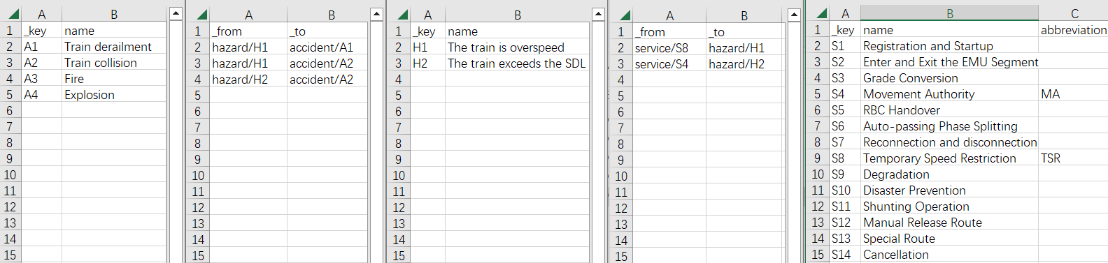
3. You can see that ArangoDB uses an individual file to correlate two collections like “Mysql”. Such isolation allows us to conveniently and accurately modify the contents of the database
- The
_fromand_toattributes of the “edge” file form the graph by referencing document_id - The
_idis automatically generated by concatenating the “collection name” and_keywith “/” while importing
Create Collections
1. Import the aforementioned CSV files one-by-one to the ArangoDB by running the following on your command-line:
- Document
arangoimport --file PATH TO ".csv" ON YOUR MACHINE --collection NAME --create-collection true --type csv
- Edge
arangoimport --file PATH TO ".csv" ON YOUR MACHINE --collection NAME --create-collection true --type csv --create-collection-type edge
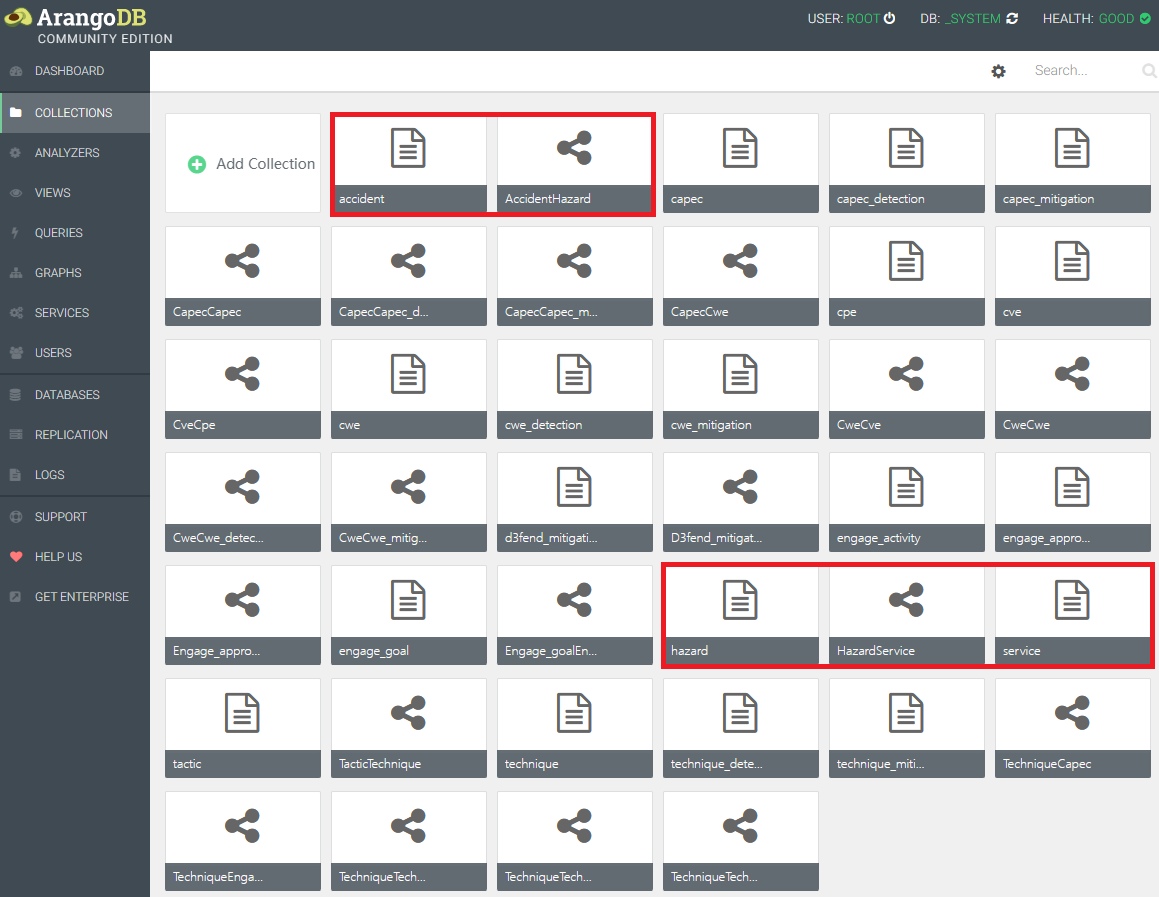
2. Results (The import processes of “Control Action”, “Weakness”, “Safety Constraint”, “Asset” and “Threat Scenario” are omitted here):

Query & Traversal
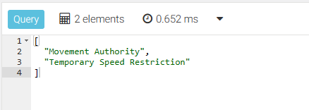
1. Query to find out how many “services” have “abbreviation”:
FOR s IN service
  FILTER s.abbreviation
  RETURN s.name
2. Query to see the relationship between “accident” and “hazard”:
FOR r IN AccidentHazard
  RETURN r

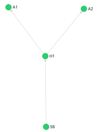
3. Traverse to check whether our collections are correlated together (start from “service/S8”):
FORvertex(, edge)(, path)IN min..maxdefines the minimal and maximal depth for the traversal (min defaults to 1 and max defaults to min)OUTBOUND/INBOUND/ANYdefines the direction of your search- The subsequent format is ‘StartVertex’ edge_collection1, edge_collection2, …
-- Traversal follows outgoing edges, only returns "accidents" caused by "S8" (Result: left pic)
FOR v, e, p IN 1..3 OUTBOUND 'service/S8' HazardService, AccidentHazard
RETURN p
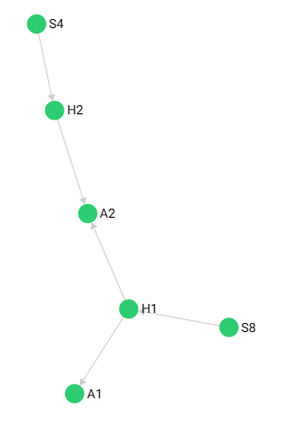
-- Traversal follows edges pointing in any direction, will return more contents like "S4" (Result: right pic)
FOR v, e, p IN 1..5 ANY 'service/S8' HazardService, AccidentHazard
RETURN p
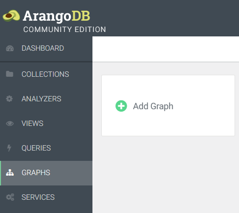
Create Graphs
1. In ArngoDB we can directly construct a graph to view the structure of our knowleges. Notice that this is only a visual tool, actually all the collections in a database are already a comprehensive graph
- The abstract structure of all POCA analysis results is shown below:

2. According to the abstract structure, we can use corresponding collections to construct the graph with ArangoDB, it is pretty simple:
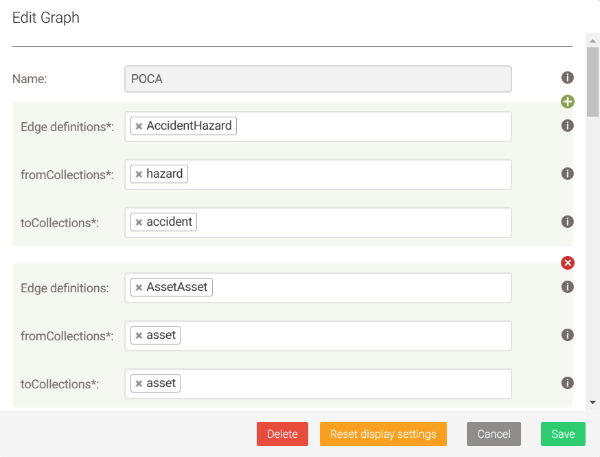
3. The final graph of the “POCA analysis results” in ArangoDB is shown below:
